

Speed Gates in Fighter Radars: Logic of Doppler Tracking
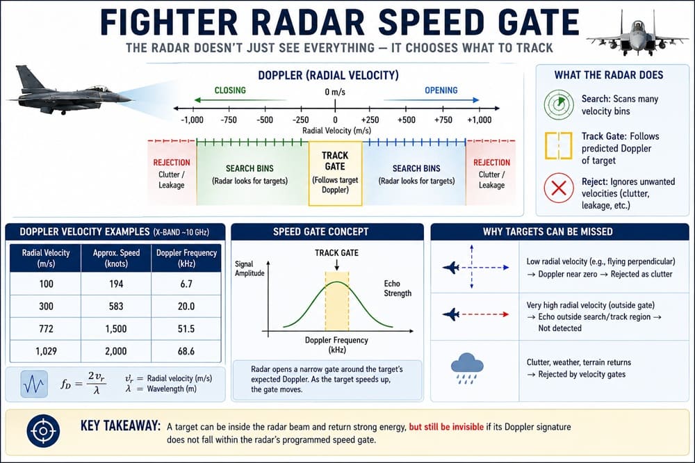
Today fighter radars are not only looking for reflected energy. They sort echoes by range, direction, amplitude and radial speed. This process relies heavily on the “speed gate”, properly referred to as the velocity gate or Doppler gate. Radar can distinguish an aircraft from terrain, weather, birds, vehicles, chaff and electronic interference. It can also miss a real target which has a Doppler signature outside the programmed processing envelope of the radar. Exact gate limits, pulse-repetition frequency timing, and rejection algorithms are classified. But the physics behind this is in the open technical literature.
Doppler Measures Radial Speed
A pulse-Doppler radar measures how rapidly the distance between the radar and target changes. It does not directly measure the target’s true airspeed. The Doppler frequency is:
f_D=\frac{2v_r}{\lambda}
Here, (v_r) represents relative radial velocity, while (\lambda) represents radar wavelength. For an X-band fighter radar operating near 10 GHz, the wavelength is approximately 0.03 metres. These figures represent closure or opening velocity along the radar’s line of sight. A fighter crossing perpendicular to that line can produce almost no target-generated radial velocity despite flying at supersonic speed.
| Radial velocity | Approximate speed | Doppler frequency |
|---|---|---|
| 100 m/s | 194 knots | 6.7 kHz |
| 300 m/s | 583 knots | 20 kHz |
| 772 m/s | 1,500 knots | 51.5 kHz |
| 1,029 m/s | 2,000 knots | 68.6 kHz |
Search Bins and Gates
The term ‘speed gate’ can refer to three related functions. The first step of the searching procedure is to divide the Doppler spectrum into a large number of velocity bins. Each bin has a finite width in frequency. The radar looks for energy above an adaptive detection threshold. Second, the radar may be programmed to ignore some velocity regions. These rejection bands reject stationary clutter, side-lobed clutter, transmitter leakage and other unwanted signals.
Third, the tracking system, once acquired, opens a narrow velocity gate centred around the predicted Doppler frequency of the target. As the target speeds up, the gate moves. And this difference counts. A search filter does not have to be a tracking gate. A radar may not acquire a target in search but may lock on to it once a track is established. “Pulse-Doppler processing is coherent integration over multiple pulses and separation into Doppler-velocity bins,” says MIT Lincoln Laboratory. It also states that airborne radars use several PRFs to suppress clutter and resolve ambiguous velocities.
Why Multiple PRFs Matter
Pulse repetition frequency determines how often the radar transmits pulses. It creates an unavoidable range-velocity trade-off. Consider an illustrative X-band radar using a 50 kHz PRF. Its unambiguous range would be:
R_u=\frac{c}{2,PRF}=3\text{ km}
Its single-PRF unambiguous radial-velocity interval would extend approximately to:
v_u=\pm\frac{\lambda,PRF}{4}=\pm375\text{ m/s}
Higher velocities are not physically gone. They fold into an ambiguous Doppler cell and can appear as a slower target or clutter. Low PRF gives good unambiguous range but poor velocity discrimination. The high PRF is good for velocity measurements but has serious range ambiguity. For medium PRF, the processor must compare several waveforms, leading to ambiguity of both measurements.
Published literature on the AN/APG-66 of the F-16A/B indicated that the medium-PRF down-look mode transmitted eight different PRFs per antenna dwell. The flight test included a head-on target to approximately 30 nautical miles, a 3-degree antenna depression angle and a 2-bar scan of +/-30 degrees. The processor cross-correlated detections across those PRFs. If they were real targets, they produced consistent solutions but ambiguous returns and normally failed the correlation test.
Velocity Resolution
Velocity resolution depends strongly on coherent processing interval, or CPI:
[Delta v\approx\frac{\lambda}{2T_{CPI}}
Theoretical velocity resolution at 0.03-metre wavelength and 20-millisecond CPI is about 0.75 m/sec or 1.46 knots. Practical performance is degraded by windowing, manoeuvres, clutter, noise and antenna scanning. CPI longer can improve the Doppler resolution, but it will cause one more trouble. During processing, a fast-manoeuvring aircraft can cross many Doppler bins. Engineers refer to this phenomenon as range-Doppler migration, or spectral spreading. Some of the migration is compensated for by modern processors. However, the radar has to compromise between sensitivity, update rate, processing load and target acceleration.
The Radar Notch
Pilots often use the term “notching” when they turn about 90 degrees away from an attacking radar. This manoeuvre reduces the radial velocity of the aircraft and puts its return near to the clutter spectrum. The explanation for an airborne radar is more complicated. The radar-carrying fighter would be moving, so the stationary terrain has a huge Doppler.
Thus, the main-lobe ground clutter produces a wide Doppler ridge, centred at the projected velocity of the radar aircraft. If the doppler return of a defending aircraft is over this ridge, it becomes difficult to distinguish. Or it may reject it with the clutter, rather than accepting thousands of ghost contacts. A perfect 90-degree turn does not guarantee safety. The required geometry changes with:
- The attacker’s speed and heading
- Antenna depression angle
- Target altitude and range
- Terrain movement and wind
- Clutter-filter width
- PRF selection
- Track memory and sensor fusion
A radar can also maintain range and angle gates after Doppler quality deteriorates. Therefore, entering the notch may weaken a track without immediately breaking it.
SR-71 Eagle Bait Case Study
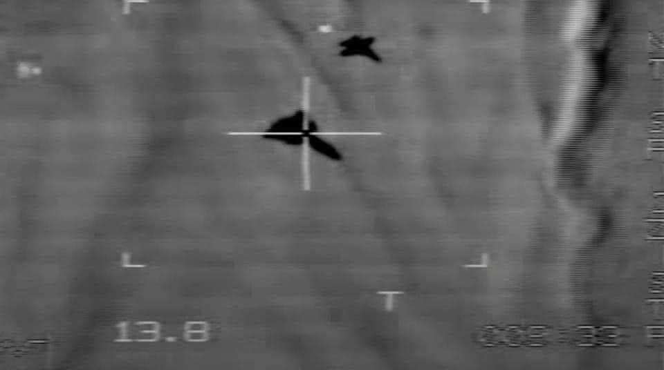
The “Eagle Bait” exercises, held in the early to mid-1980s, uncovered an odd limitation in velocity processing. In a controlled environment, the SR-71 gave F-15 crews a chance to practise against an extremely fast target at a very high altitude. “F-15 crews frequently had trouble finding the Blackbird, even when they knew where it was headed,” former SR-71 pilot Dave Peters said.
The problem was blamed on a reported speed-gate limit of 1,500 knots, but the SR-71 was producing a speed of around 1,850-2,000 knots as relevant. This corresponds to a Doppler shift of ~51.5-68.6 kHz at X-band. A processor programmed to look only in a lower Doppler region might have rejected the SR-71 before it was displayed. The exercises were said to require prior knowledge, good positioning and disabling the electronic countermeasures of the Blackbird. But crews still had trouble conducting simulated engagements.
Published account of the Eagle Bait sorties. However, that exact 1,500-knot figure should give analysts pause. There is no APG-63 engineering document released to the public that verifies that. Peters’ story likely relates to a specific radar mode, software setting, or an accepted velocity window, not the hard physical limit of all f-15 radars. The important lesson still applies: a powerful radar can get a strong echo but reject it because the signal doesn’t fit its programmed threat model.
Electronic Attack on the Gate
The speed-gate pull-off exploits this tracking logic. A coherent jammer produces a false return at the target’s true Doppler frequency. Then slowly it alters that frequency. If the false signal is stronger, the tracking loop will track that signal. Finally the real aircraft departs the gate, and the radar sees the wrong velocity. The published literature on early semi-active missile seekers mentions typical speed-gate bandwidths of 500 Hz to 2 kHz.
At a wavelength of three centimetres, this corresponds to a radial velocity width of about 7.5-30 m/sec or 15-58 knots. Public reference engineering radar seekers Current systems counter this method with range-Doppler consistency checks, acceleration constraints, monopulse angle tracking, multi-PRF validation, inertial track prediction and data from other sensors.
Operational Meaning
So detection by radar is not just a matter of transmitter power vs radar cross-section or Speed gates. The processor has to decide which returns to focus on. The combat record of the F-15 shows that Doppler limits can be overcome; they are not insurmountable. F-15Cs accounted for 34 of the U.S. Air Force’s 37 air-to-air kills in Desert Storm. A pulse-Doppler radar enabled it to attack targets above and below the fighter.
U.S. Air Force Modern AESA radars have improved waveform agility, processing speed, track memory and clutter adaptation. They do not negate the physics of Doppler. Each radar still has to decide what velocities to look for, reject and track. The most important and often forgotten fact is a target can be inside the antenna beam, can be returning enough energy, but still not be visible to the pilot. The radar software may deliberately decide the echo could not be a valid aircraft.
References
- Ringel, M. B., Mooney, D. H., & Long, W. H. III. “F-16 Pulse Doppler Radar (AN/APG-66) Performance.” IEEE Transactions on Aerospace and Electronic Systems, Vol. AES-19, No. 1, 1983, pp. 147–158. The paper covers medium-PRF clutter, signal processing, flight testing, detection and false-alarm performance.
- Long, W. H., & Harriger, K. A. “Medium PRF for the AN/APG-66 Radar.” Proceedings of the IEEE, Vol. 73, No. 2, February 1985, pp. 301–311. Particularly relevant to multiple-PRF processing and range/Doppler ambiguity resolution.
- Graham, Richard H. The Complete Book of the SR-71 Blackbird. Voyageur Press, 2015. Provides first-hand and historical material on SR-71 operations, performance and fighter-intercept exercises.
- U.S. Air Force. “F-15 Eagle.” USAF Fact Sheet. Includes the F-15’s radar/avionics role and confirms that F-15Cs scored 34 of the USAF’s 37 air-to-air victories during Operation Desert Storm.
About the Author



1 thought on “Speed Gates in Fighter Radars: Logic of Doppler Tracking”